The Middle East and North Africa (MENA) region suffers from both, data availability and data quality. Any effort to collect, clean and present data on the region is a welcome initiative.

Economena Analytics is doing just that. Economena collects data on many indicators in the MENA region and presents them in a way that is easily accessible for policy makers, researchers and academics. In this blog, we extract data on Dubai International Airport passenger traffic from the Economena Analytics Online Databases to illustrate Stata’s graphics abilities.

The data we have is monthly numbers of passengers at Dubai International Airport divided into three main categories: arriving passengers, departing passengers and transit passengers all in thousands. We limit the data from January 2000 to December 2014. We then use the year() and month() functions to separate the month and year from the date variable downloaded. We now have two new variables that identify the month and year of each observation. This is helpful if I want to perform any analysis specific to a month or year (for instance collapsing by a certain month or year).

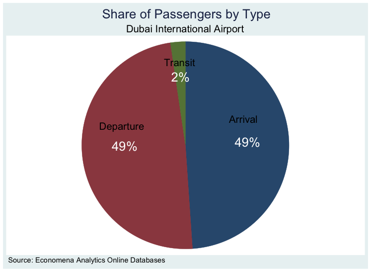
We will first create a pie graph that shows the share of each type of passenger from the overall number of passengers. The pie graph is below and tells us that transit passengers only account for 2% of the total number of passengers at Dubai International Airport. Both departing and arriving passengers make up an equal 49% share of the total number of passengers. Note here that I intentionally added the shares to the graph in white while keeping the labels in black. I could have changed both colours to match each other or to any different colour. The same applies to the colours of the slices. We could have also separated the slices from each other.


We now move to the second graph which is a line plot graph with connected lines. In this graph, We show three data series: the mean share of arrivals, departures and transit passengers by year. To get the mean shares We used the collapse command in Stata. The blue and dark red lines represent the arrivals and departures and the left hand y-axis should be used to read their values. The green line represents the transit passengers and the right hand y-axis should be used to read its values.


The graph says that in 2000, transit passengers were around 10% of the total passenger traffic at Dubai International Airport but this share has decreased all the way to less than 1% starting in 2012. On the other side, arrivals and departures have consistently increased over the first 14 years of the 3rd millennium going from around 45% in 2000 to almost 50% in 2014. Both of these suggest that Dubai is a destination city rather than a transit city.

I have showed different symbols (circle, triangle and square) for the lines, using the msymbol() function in Stata, to allow easier reading of the graph in case it was printed in non-color format.
Finally, we also added a vertical dashed red line for year of the financial crisis (2008). The line shows a drop in the share of arrivals to Dubai between 2008 and 2009 of around 2.5%. The share of arrivals did recover increasing between 2009 reaching a new peak in 2012 (where we added another vertical dashed red line). The new peak in 2012 is slightly lower than that of 2008. Interestingly, the share of departures suddenly jumped between 2008 and 2009. Note here that We am talking about the share of arrivals and departures and not the number of passengers as arrivals or departures. To look at the total number of arrivals and departures it would be good to graphs these using dates. We suggest using the tsline command to plot time-series data.
The above exercise was a simple implementation of data management and Stata graphics using data from Economena Analytics. For the Stata dofile of this exercise click here. If you would like to learn more about how to deal with data in Stata, see the list of the upcoming Timberlake Stata courses.

George Naufal @georgenaufal

Often in data work one finds that the same work needs to be done again and again. Repeated actions and steps are an ideal reason to resort to programming capabilities of statistical software. In other terms, if one can get the computer to do the work that can be automated, one increases efficiency with regards to time but also to avoid errors. To summarise, one should always rely on computers and software to perform repetitive tasks. This saves time, is more efficient and prone to less mistakes.

A common task is to rename or create new variables, often a large number of variables. In this exercise, we use a fictional dataset to provide a simple example of how to use the programming capabilities of Stata to create several variables.

The data set is called “rain data” and includes rain precipitation numbers (in inches) for 10 cities between 2000 and 2003.

Download the data here.

First, you would like to create a variable that list the highest precipitation record across the 4 course by city. One could look at each row and copy the highest number. This obviously is not feasible, prone to mistakes and is time consuming (just imagine the data set includes 1000 cities!). I use the egen command in Stata with the rowmax function to push Stata to search across each row (so each city) and return the maximum number and place it in the new variable. The command egen is very powerful with a large number of functions that are very useful.

Assume now that you would like to create a variable for each year and each city that is 1 if the rain precipitation is higher than 35 inches (and 0 otherwise). Because the data set includes 4 years of rain precipitation data (2000, 2001, 2002 and 2003) I will have to generate 4 new variables. Creating 4 new variables can be done through the generate command using the if qualifier. This would take 4 lines of code. If I want to label each new variable then this will take another 4 lines. However, imagine the data set included 40 years of data, then this become cumbersome and a source of potential errors with more than 80 lines of code! I use the forvalues loop to push Stata to run through the years 2000 to 2003, generate 4 new variables with the condition of rain precipitation above 35 inches and also to label each variable. The command forevalues sets a macro name to each element of a range and executes the commands enclosed in brackets. In this case, the enclosed commands in brackets are “generate 4 new variables and also label the new variables”. The loop accomplishes the same task in 3 lines of code (instead of 8) and with a much higher accuracy (in terms of avoiding human errors in repeated tasks).

Download the Stata do-file of this exercise here.

The use of Bayesian analysis is on the rise and is widespread across different disciplines including health, medicine, economics and other social sciences. The main difference of Bayesian analysis over the classical, frequentist method, is that a Bayesian assumes model parameters to be random and therefore having distributions while the frequentist method assumes model parameters to be unknown but fixed. Under Bayesian, one relies on a prior knowledge for the unknown and uses evidence from observed data (likelihood model) to get a posterior distribution of unknown parameter. The main advantages of the Bayesian approach is the ability to include prior information in the analysis. It also allows researchers to better handle repeated, missing, unbalanced and multivariate data.

Stata 14 offers 12 built-in likelihood models for different outcomes (continuous, binary, ordinal and count), the capability to write own likelihood models and the ability to use the 22 built-in priors and to take advantage of postestimation features. A new command, bayesmh, allows users to fit models using two different algorithms (Metropolis-Hastings algorithm, Gibbs algorithm or a combination of both) for univariate, multivariate and multiple-equations, both linear and nonlinear.

Upgrade your Stata license to learn more about Bayesian analysis with the all-new 261 page Stata Bayesian Analysis Reference Manual that is part of Stata 14’s extensive documentation.

This month, our latest edition of Stata Tips, Timberlake Group Technical Director, Dr. George Naufal shares his thoughts and insight on the Project Manager features available in Stata.

PROJECT MANAGER

Often researchers find themselves collaborating on empirical projects. Colleagues at research and government institutions frequently work together on data based projects. From analysing the data to presenting the findings, it is not uncommon to create several files of different types: data files, data visualisation files, log files, do-files and output files. Depending on the size of the data and the scope of the project, the number of generated files could be substantial (hundreds if not even thousands).

Project Manager in Stata offers the capability to integrate all of the files from a specific project (or even multiple projects) into one location that can easily be shared among collaborators. ‎Project manager includes the option to filter following filenames; create folders within folders and to open files within Stata.

Project Manager is not only ideal for collaborations between researchers, it is also a great tool for the classroom. Instructors can organise their data sets, do-files for practical exercises, exams and even lecture notes.

With the rich documentation in Stata 13, you can learn more about how to organise your empirical projects using the Project Manager.

Additionally, all of our Stata public attendance training courses also teach users to get the most out of the the Project Manager. In beginner courses, our course instructors help delegates organise and edit data, while more advanced topics identify how users can collaborate on single and multiple projects.

TOUR OF PROJECT MANAGER Explore the new Project Manager in Stata 13. The Project Manager allows us to easily organize, view, and edit our data, programs and graphs.